Robust fitting via Latin Hypercube sampling (LHS)
Classes used:
Instead of using informed guesses for the initial values of the variable parameters of a model, these initial values are randomly chosen using a Latin Hypercube. For each of the resulting grid points, an optimisation is performed, analogous to what has been described above.
Generally, this approach will take much longer, with the computing time scaling with the number of grid points, but it is much more robust, particularly with complicated fitness landscapes containing many local minima.
Recipe
 1format:
 2  type: ASpecD recipe
 3  version: '0.2'
 4
 5settings:
 6  autosave_plots: false
 7
 8tasks:
 9  # Create "dataset" to fit model to
10  - kind: model
11    type: Zeros
12    properties:
13      parameters:
14        shape: 1001
15        range: [-10, 10]
16    result: dummy
17    comment: >
18        Create a dummy model.
19  - kind: model
20    type: Gaussian
21    from_dataset: dummy
22    properties:
23      parameters:
24        position: 2
25      label: Random spectral line
26    comment: >
27        Create a simple Gaussian line.
28    result: dataset
29  - kind: processing
30    type: Noise
31    properties:
32      parameters:
33        amplitude: 0.2
34    apply_to: dataset
35    comment: >
36        Add a bit of noise.
37  - kind: singleplot
38    type: SinglePlotter1D
39    properties:
40      filename: dataset2fit.pdf
41    apply_to: dataset
42    comment: >
43        Just to be on the safe side, plot data of created "dataset"
44
45  # Now for the actual fitting: (i) create model, (ii) fit to data
46  - kind: model
47    type: Gaussian
48    from_dataset: dataset
49    output: model
50    result: gaussian_model
51
52  - kind: fitpy.singleanalysis
53    type: LHSFit
54    properties:
55      model: gaussian_model
56      parameters:
57        fit:
58          position:
59            lhs_range: [-8, 8]
60        lhs:
61          points: 70
62    result: fitted_gaussian
63    apply_to: dataset
64
65  # Plot result
66  - kind: fitpy.singleplot
67    type: SinglePlotter1D
68    properties:
69      filename: fit_result.pdf
70    apply_to: fitted_gaussian
71
72  # Extract statistics and plot them
73  - kind: fitpy.singleanalysis
74    type: ExtractLHSStatistics
75    properties:
76      parameters:
77        criterion: reduced_chi_square
78    result: reduced_chi_squares
79    apply_to: fitted_gaussian
80
81  - kind: singleplot
82    type: SinglePlotter1D
83    properties:
84      properties:
85        drawing:
86          marker: 'o'
87          linestyle: 'none'
88      filename: 'reduced_chi_squares.pdf'
89    apply_to: reduced_chi_squares
90
91  # Create report
92  - kind: fitpy.report
93    type: LaTeXLHSFitReporter
94    properties:
95        template: lhsfit.tex
96        filename: report.tex
97    compile: true
98    apply_to: fitted_gaussian
Result
The two first figures created in the recipe, namely those of the data and the fit results, are basically identical to the previous example given for fitpy.analysis.SimpleFit and are hence omitted here. Instead, the result of plotting the chi suqare values to assess the robustness of the LHS approach is shown below.
While in the recipe, the output format has been set to PDF, for rendering here the figure has been converted to PNG. Due to the LHS having an inherently random component, your figure will look different. Nevertheless, you should get the overall idea of such plot for assessing the robustness of a fit employing LHS.
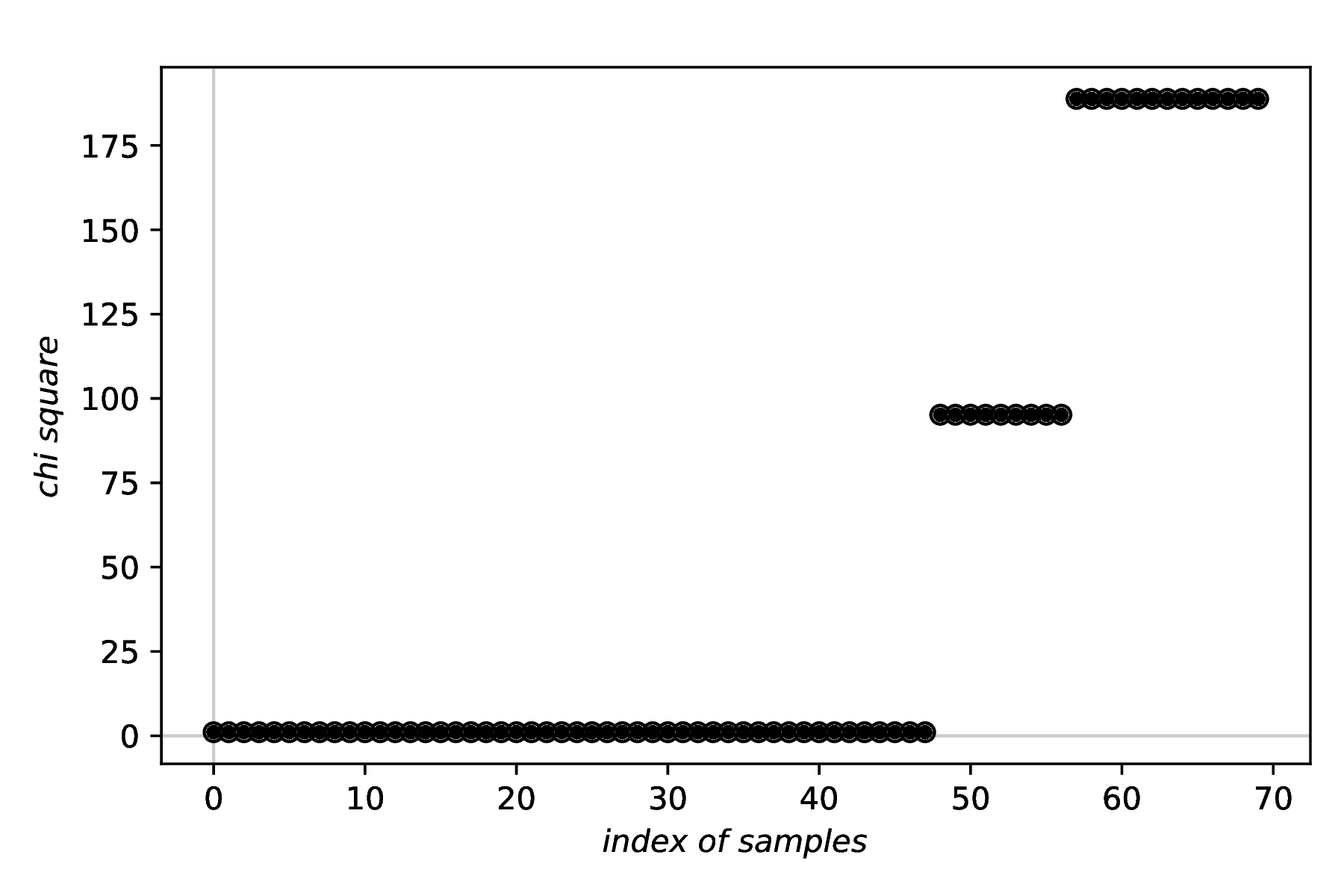
Robustness of the fit. As generally fitting is a minimisation problem, the lower the value of the respective criterion, the better the fit. For a rough fitness landscape, you will likely observe several plateaus, and ideally a visible plateau at the very left, representing the lowest (hopefully global) minimum.
Comments
The purpose of the first block of four tasks is solely to create some data a model can be fitted to. The actual fitting starts only afterwards.
Usually, you will have set another ASpecD-derived package as default package in your recipe for processing and analysing your data. Hence, you need to provide the package name (fitpy) in the
kindproperty, as shown in the examples.Fitting is always a two-step process: (i) define the model, and (ii) define the fitting task.
To get a quick overview of the fit results, use the dedicated plotter from the FitPy framework:
fitpy.plotting.SinglePlotter1D.To assess the robustness of the fit and the LHS strategy, extract one statistical criterion from the data using
fitpy.analysis.ExtractLHSStatisticsand afterwards plot the results using a standard plotter from the ASpecD framework.For a more detailed overview, particularly in case of several fits with different settings on one and the same dataset or for a series of similar fits on different datasets, use reports, as shown here using
fitpy.report.LaTeXLHSFitReporter. This reporter will automatically create the figure showing both, fitted model and original data, as well as the figure allowing to assess the robustness of the fit.